Page Contents
Pressure Plots
MAPP 3D provides two different methods to evaluate the performance of a system design:
- The first shows sound pressure distribution on geometry for a narrow range of frequencies—up to one octave wide—in the Model View tab. These are often referred to as pressure plots.
- The second is to add virtual microphones to the model in strategic locations to evaluate the broadband response and maximum acoustic output. See Measurement View.
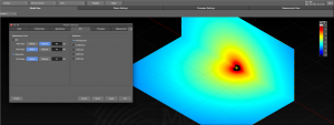
Pressure plots displayed on geometry in the Model View tab enable visualization of coverage and loudspeaker to loudspeaker interactions on any geometry selected for prediction. A pressure plot can be up to one-octave wide, a periscope view of the entire band spectrum. Below, the image on the left is a one-octave wide prediction, centered at 4 kHz. The data from the microphone location in the Model View (left, below) is represented in Measurement View (right, below). When the prediction bandwidth is one octave, the data points highlighted in the Measurement View are averaged and the level is represented using colors in the Model View.
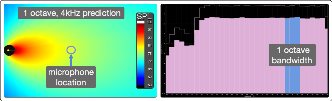
Model View Periscope View of Bandwidth (left) and Measurement View, One Octave, Centered at 4 kHz, Highlighted (right)
Generally, a one-octave prediction at 4 kHz is representative of high frequency coverage. A one-octave prediction at 250 Hz is representative of mid-band frequencies. As frequency decreases to the subwoofer range, 1/3-octave predictions from 100 Hz down to the lowest frequencies the system reproduces are effective to analyze coverage and loudspeaker-loudspeaker interactions.
Prediction planes are acoustically transparent in the model, except geometry selected as Ground Plane. See Ground Plane.
The graphic representation of sound pressure in MAPP 3D has several parameters located on the main application window and in the FILE > PROJECT SETTINGS menu, both on the Appearance and SPL tabs. These are described below.
Model View Pressure Plots
To generate a pressure plot on geometry, the model must include:
- at least one loudspeaker on a visible layer
- at least one prediction plane (geometry selected for Prediction) on a visible layer
- processor channel must be assigned and un-muted with level above -∞ dB
Make the below selections for a prediction:
- generator level

- signal type

- width of prediction, up to one octave

- range of frequencies – no options when width is one octave
- center frequency

Click PREDICT (cmd-R) to generate a pressure plot on the prediction planes. Click CLEAR to remove pressure plot from prediction planes.
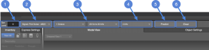
Model View Tab, Prediction Parameters
Signal Generator
The generator level and signal type affects the SPL results.
The generator level is adjustable between -90 dB and +50 dB.
The generator signals available are:
- Pink Noise is generated by SIM, which has a 12.5 dB difference between peak and average levels (crest factor).
- B-Noise is SIM pink noise filtered with a B-weighting curve. Use B-Noise to more accurately predict the maximum output of a system when speech is the input signal.
- M-Noise is a signal that closely represents the peak-to-average ratio as a function of frequency expected of music, currently under consideration by an AES standards committee. Below 500 Hz Pink Noise and M-Noise are functionally the same. For more information, please see M-Noise.org.
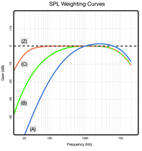
Weighting Curves – A, B, C, and Z
SPL Tab Parameters
Adjust the Project Settings parameters to change how pressure plots are displayed. Use the FILE > PROJECT SETTINGS menu (cmd-shift-P) and select the SPL tab to access these settings.
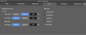
Project Settings – SPL Tab
SPL Scaling
When SPL is selected, the average SPL (not peak) is represented by colors for the selected bandwidth. The default range and value settings can be changed by clicking the MANUAL buttons (above) and entering new values.
The Max Value is the loudest level plotted. If levels exceed this value, the area is plotted white. Increase the Max Value until white is no longer displayed, see below.
The Min Range is the number of dB below the Max Value that will be plotted. If the prediction plane is plotted black, the SPL values are below the level range plotted. To plot as colors other than black, decrease the Max Value or increase the Min Range value, see below.
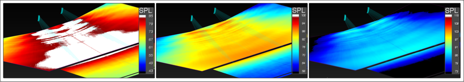
Model View – SPL, Change Only to Max Value Level: 85 dB (left), 100 dB (middle), and 115 dB (right)
When a loudspeaker is predicted with the Max Value = 75 dB, SPL values of 70 dB are plotted as red, (1) below. When the Max Value is set to 87 dB, 70 dB is plotted as yellow, (2) below. It’s the same data, just scaled and plotted differently.
For (2) below, when the Range = 42 dB, 42 dB of attenuation below the Max Value of 87 dB is plotted. In (3) below, when the Range = 30 dB, levels between 87 dB and 57 dB are plotted. 70 dB is now plotted as a light blue color. Again, it is the same data, just scaled and displayed in different way.
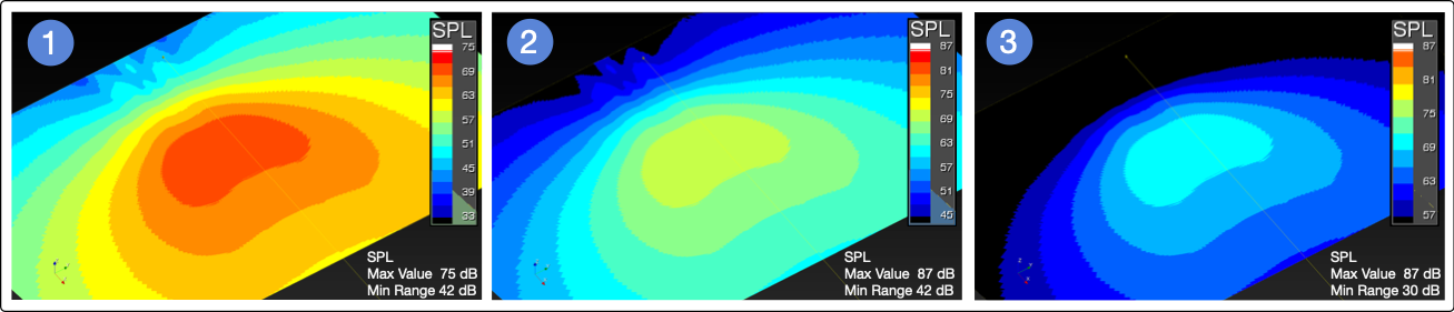
Model View Predictions, SPL Mode – Same Data Represented Differently Based on SPL Max Level and Min Range Settings
The SPL values are only for the range of frequencies selected. When narrower prediction bandwidths are selected, the SPL values decrease. The pressure plots below use the same parameters for the same loudspeaker, the only change is the bandwidth of the prediction.
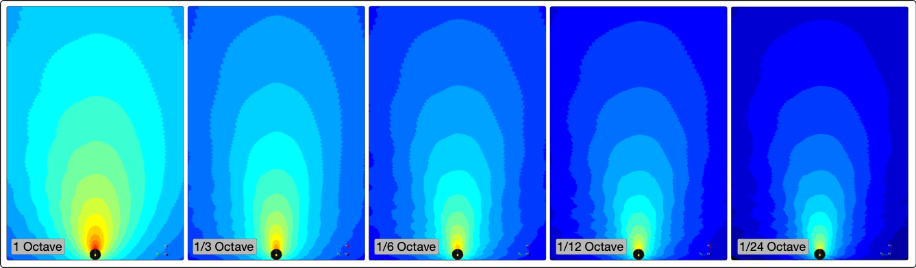
Model View, SPL – Less SPL as Bandwidth Narrows
Resolution
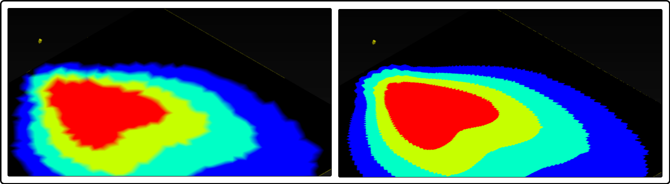
Resolution determines the number of colors used to represent pressure. Select Full Resolution, or level deviation per color used. The number of colors used to plot SPL or Attenuation can be helpful in different ways. Full Resolution uses a large number of colors to represent pressure, which are impressive images to include with a proposal. Using the 3 dB/color or 6 dB/color resolution settings makes determining coverage areas more obvious.
When changing between resolutions, no re-calculation is performed, the application only re-renders the prediction data.
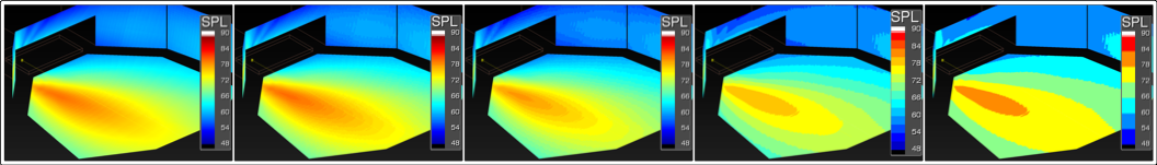
Model View – Resolution Settings, Full Resolution, 0.5 dB, 1 dB, 3 dB, and 6dB Per Color
Attenuation Range
The Attenuation selection uses colors to represent attenuation, normalized to the point on all of the prediction planes that has the highest pressure level. The color at the top of the scale (0 dB) represents this point. All other points are equal or less in level, represented by colors indicating level of attenuation.
To modify the range of SPL represented, click MANUAL and enter a higher or lower range of attenuation to display. This is the level of attenuation from 0 dB that will be plotted.
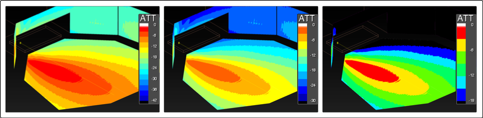
Model View – Attenuation, Min Range 42 dB, 30 dB, and 18dB
Attenuation Examples
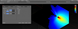
When using Attenuation mode, the level is relative to the loudest source. It is not intuitive that a subwoofer predicted at one-octave, 4 kHz appears to be very loud (below). It is in fact 30-40 dB lower in level at 4 kHz than within its operating range. Because the subwoofer is the loudest source in the model at this range of frequencies, the 0 dB color is plotted nearest this loudspeaker.
Model View – Subwoofer Prediction, One-Octave, 4 kHz
If a small, full-range loudspeaker (MM-4XP) is added to the model, the 0 dB color is plotted nearest the full-range loudspeaker because it is much louder than the subwoofer at 4 kHz.
Model View – Subwoofer and Mid-High Loudspeaker Prediction, One-Octave, 4 kHz
Appearance Tab Parameters
Adjust the Project Settings parameters to change how pressure plots are displayed. Use the FILE > PROJECT SETTINGS menu (cmd-shift-P) and select the APPEARANCE tab to access these settings.
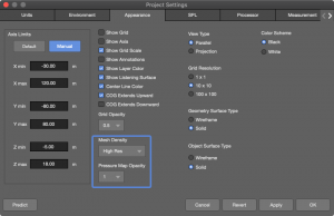
Project Settings – Appearance Tab, Mesh Density and Pressure Map Opacity
Mesh Density
The Mesh Density selection determines the resolution of the SPL map, and affects both calculation time and how detailed the pressure plot will be. A higher density has more points on the listening planes, creating a highly detailed pressure plot that takes longer to calculate than a lower mesh densities (see below).
Model View Prediction – Mesh Density Setting Very Low (left), Very High (right)
Pressure Map Opacity
Pressure Map Opacity changes the opacity of the prediction data in the Model View tab, 1.0 is opaque, 0.1 is almost transparent. (see below).
Model View – Pressure Map Opacity 1.0 and 0.7
Data Near Loudspeaker
Each loudspeaker data set has a small data void around the loudspeaker, intentionally.
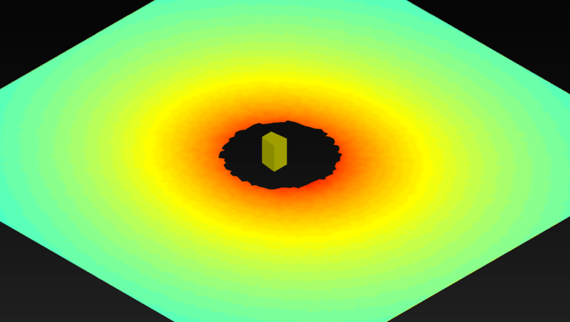
Model View – Data Not Available Within One Meter
Example Uses
Example 1: The Model View image below is of a one-octave, 4 kHz, 3 dB/color prediction. The colors indicate level on-axis ![]() , -3 dB down
, -3 dB down ![]() , -6 dB down
, -6 dB down ![]() for the octave centered at 4 kHz. When in SPL mode, the SPL values are for the bandwidth of the prediction only, one octave in this case. Relative pressure levels are available in Attenuation mode, the same as in MAPP XT.
for the octave centered at 4 kHz. When in SPL mode, the SPL values are for the bandwidth of the prediction only, one octave in this case. Relative pressure levels are available in Attenuation mode, the same as in MAPP XT.
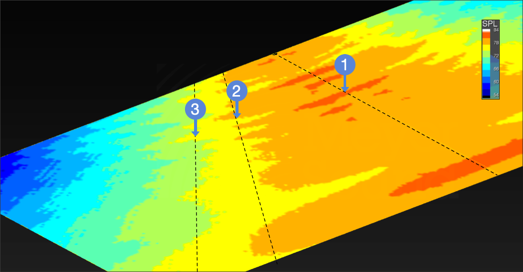
Model View – One Octave, 4 kHz, 3 dB/Color, SPL Prediction – On-Axis (1), -3 dB (2), -6 dB (3)
Example 2: To evaluate coverage of a loudspeaker model using a standard level of variance for designs, +/- 3 dB or 6 dB, one option is to select Attenuation, Min Range = 12 dB. The first two colors indicate where coverage is within the design limits. The center of the red area is relative 0 dB. Between the red and yellow color is 3 dB less level. Between the yellow and green color is another 3 dB less level.
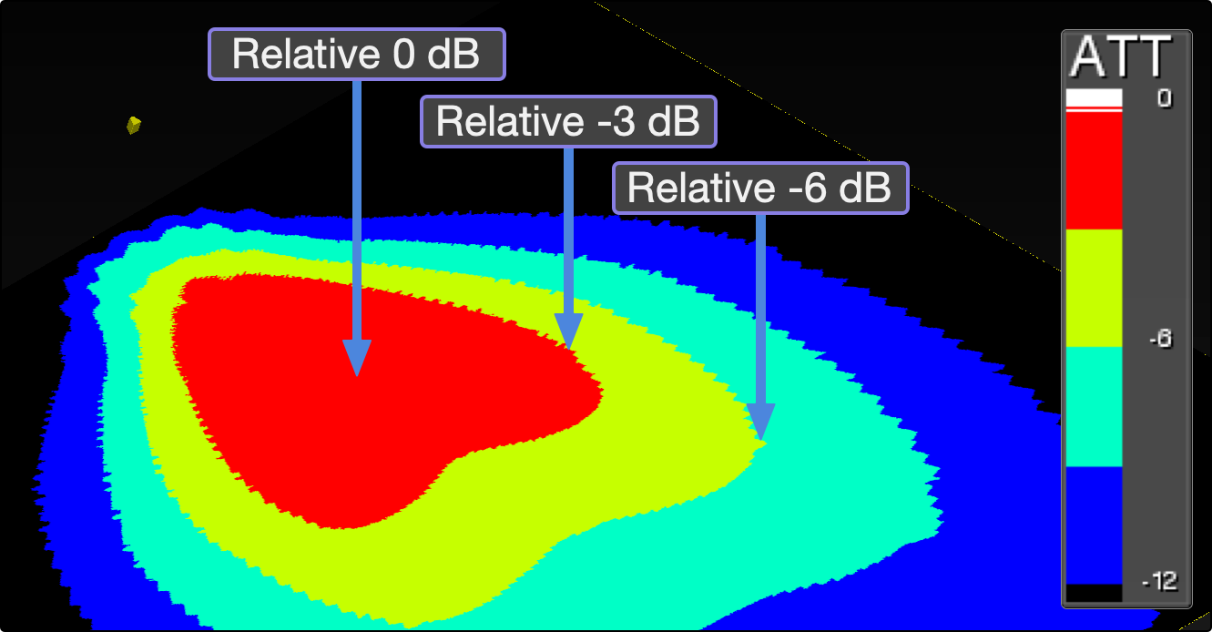
Model View – Attenuation, Range = 12 dB, Colors Represent Relative Level
Below, three different loudspeaker models are evaluated with slight location and aiming changes. On the left, the coverage is too narrow, even if the loudspeaker were better aimed. In the middle, there is too much level variation from front to rear. On the right, almost the entire half of the seating area is within 6 dB for the octave centered at 4 kHz. Fills may be necessary for rear of seating. For model selection, placement, and aiming, this viewing strategy is efficient.
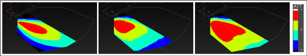
Model View – Attenuation, Range = 12 dB, Evaluate Loudspeaker Location, Orientation, and Model Selection for Coverage
What’s Next?
Please see Measurement View next.