Page Contents
Measurement View
MAPP 3D provides two different methods to evaluate the performance of a system design:
- The first is by showing sound pressure distribution over listening planes for a narrow range of frequencies—up to one octave wide—in the Model View tab. See Pressure Plots.
- The second is to add virtual microphones to the model in strategic locations to evaluate the broadband response and maximum acoustic output. This option is described below.
Analysis using only one of these methods is only partial analysis. Although it is true that most design work can be effectively accomplished using only Measurement View data, Model View predictions can inform microphone placement and help identify instances of coverage beyond the audience area(s).
To display prediction data in the Measurement View tab, at least one loudspeaker and one microphone must be added to the model.
Add Microphones
Microphones are added to display broadband information and SPL values at the microphone locations.
INSERT > MICROPHONE or right-click in model, select INSERT MICROPHONE.
Use a Z-axis value representative of an average ear height.
Once inserted, microphones can be moved, copied, arrayed, mirrored, etc., in the same ways the geometry and loudspeakers are modified.
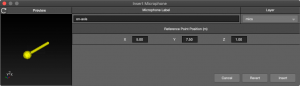
Insert Microphone Window
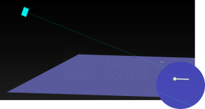
Model View – Microphone with Loudspeaker and Geometry
Microphone Placement
There are many ways to approach system design and optimization; some provide more repeatable and homogeneous coverage results than others. Microphone placement is driven by design and optimization methodology. Below are some typical microphone placement methods.
Line Arrays: Generally, microphones are placed incrementally on-axis of a line array, at least at the beginning, middle, and end of coverage. For deeper coverage areas, additional microphones are placed incrementally.
Point Source Arrays: Generally, microphones are placed on-axis to the first element, at the -6 dB point1 of the first element, and on-axis of the adjacent array element.
Fills: Generally, on-axis to the larger system, at the -6 dB point1 of the larger system, and on-axis to the fill loudspeaker.
NOTE: 1Within the range of frequencies that are directional, usually reproduced by a horn, generally 2 kHz to 20 kHz.
Frequency and IFFT Response (SIM)
The Measurement View tab is based on the architecture and nomenclature of Meyer Sound’s SIM dual-channel FFT measurement platform, which is used in our anachoic chamber to collect data for MAPP 3D.
Frequency and IFFT Response (SIM) Tab Overview
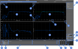
Measurement View Tab – Frequency & IFFT Tab
Measurement View – Frequency & IFFT, Pane View Selection Options
Frequency & IFFT Response (SIM) Signal Patching
A transfer function is the difference between two signals. In order to compare them, the signals compared must be synchronized. Delay is added to the generator signal and to the processor signal to synchronize them with the microphone signal. This delay is added in MAPP 3D by clicking the Propagation Delay AUTO button. The delay time is displayed next to the AUTO button. A delay time can also be manually entered here.
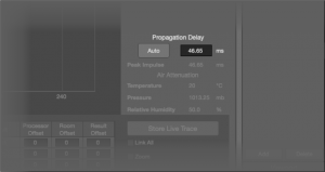
Measurement View, Frequency & IFFT Response Tab – Auto Propagation Delay
Three transfer functions are available: Processor, Speaker+Room, and Result, which are depicted below and used in MAPP 3D.
NOTE: In MAPP 3D, “Room” is the same as “Speaker + Room” used below.
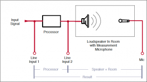
SIM Signal Patching and Transfer Function Names
For devices (processors and loudspeakers) that have the same performance at low and high levels, the transfer functions do not change for broadband, high density (not sparse) signals like pink noise, B-Noise, and M-Noise, which are selectable as the generator signal in MAPP 3D. The loudspeaker data sets in MAPP 3D are stored at the onset of limiting, the boundary of linear operation, which we use as the definition of maximum acoustic output.
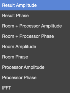
The views available in the Frequency Response & IFFT panes are (defaults in bold):
- Result Amplitude: the amplitude transfer function between the processor input and the microphone
- Result Phase: the phase transfer function between the processor input and the microphone
- Room Amplitude: the amplitude transfer function between the processor output and the microphone
- Room Phase: the phase transfer function between the processor output and the microphone
- Processor Amplitude: the amplitude transfer function between the input and output of the processor
- Processor Phase: the phase transfer function between the input and output of the processor
- Room + Processor Amplitude: the Room and Processor amplitude transfer functions displayed in the same plot
- Room + Processor Phase: the Room and Processor phase transfer functions displayed in the same plot
- IFFT: the Inverse Fast Fourier Transform, or the impulse response. Only available as the difference between source and the microphone (Result), which includes the processor, loudspeaker, and air propagation time.
Frequency and IFFT Data Usage
Observe the Result Amplitude trace as equalization and level adjustments are made if there is a target system response curve. The Result curve represents the spectral balance difference between the processor input and the loudspeaker output. If the Result trace is equal amplitude (flat), the system response will represent the input without changing the spectral balance. The proper spectral balance of a system is variable, usually based on a specification or a user’s expectation. It should be determined what the desired spectral balance of system is before committing to a design. Ensure the design has enough available headroom to reproduce the spectral content at the desired or specified level without exceeding available headroom.
Observe the Room + Processor Amplitude with the processor inverted for more precise equalization. Adjust equalization filters to match the inverted Processor trace to the Room trace; the Result will be equal amplitude (flat). It is not recommended to make equalization choices from only one microphone location for most applications. One exception would be a small control or listening room where there is only one primary listener.
Use the IFFT to synchronize arrivals of different sources:
- measure, synchronize, and store the trace of the source that arrives latest in time
- recall this trace (lower-left of window under Trace Name)
- mute the first source, unmute the second source
- click the AUTO button
The difference between the stored Propagation Delay (listed in the stored trace under Result) and the current Propagation Delay is the delay time to enter in the processor channel for the earlier arriving source to synchronize the two sources.
Signal Generator
The generator level and signal type affects the SPL results.
The generator level is adjustable between -90 dB and +50 dB.
The generator signals available are:
- Pink Noise is generated by SIM, which has a 12.5 dB difference between peak and average levels (crest factor).
- B-Noise is SIM pink noise filtered with a B-weighting curve. Use B-Noise to more accurately predict the maximum output of a system when speech is the input signal.
- M-Noise is a signal that closely represents the peak and average signals present in music. Currently under consideration by an AES standards committee. For more information, please see M-Noise.org.
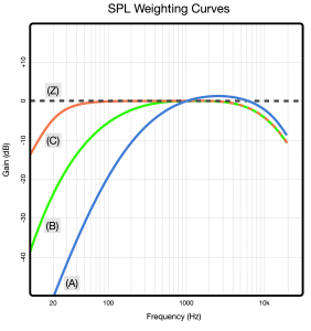
Weighting Curves – A, B, C, and Z
View Options
Click-drag in any pane to display horizontal and vertical axis values.
Select ENABLE WINDOW CENTERING to vertically center amplitude plots.
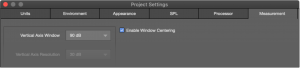
Select Enable Window Centering to Plot Traces at Vertical Center
The LINK ALL option links the Zoom and Pan settings for all like traces. All amplitude plots will have their Zoom/Pan settings linked. All phase plots will have their Zoom/Pan settings linked.
Zoom enables the use of the mouse wheel to zoom in/out of any pane.
Pan enables click-drag panning within a pane to view the entire plot when zoomed in.
Trace Display
Up to five traces can be displayed in the data plots at the same time: the live trace and four previously stored traces. Each trace will be identified by the selected Output Channel, Microphone, and Propagation Delay. Enter offset values in dB for any trace.
Trace Management
TOOLS > TRACE MANAGEMENT
Traces can be deleted by opening the Trace Management window from the Tools drop-down menu. Select the trace(s) to delete, click DELETE. When traces are stored, both the Frequency & IFFT and the Headroom data is stored using one name.
Headroom Tab Overview
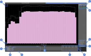
Measurement View Tab – Headroom Tab
Trace Toggles
Make selections to show/hide available traces.
- Show Peak Spectrum
- Show RMS Spectrum
SPL Values
The SPL values are dependent on signal generator level and signal type selected.
- Average SPL (A-weighted) – broadband pink noise or B-Noise value
- Average SPL (C-weighted) – broadband pink noise or B-Noise value
- Average SPL (Z-no weighting) – broadband pink noise, B-Noise or M-Noise value
- Linear Peak SPL – broadband pink noise, B-Noise or M-Noise value
- Max Linear Peak SPL – ultimate broadband peak SPL that can be achieved if all elements of the system are phase matched and time aligned to the microphone position. This is a static value, unchanged by Generator level adjustments or processor output gain adjustments. While this is not a realistic operational level, it is helpful when determining whether a loudspeaker system is capable of achieving a specified SPL value.
Headroom Data
The Headroom tab is used to determine the maximum SPL by 1/3 octave band and broadband output. This measurement is a single ended measurement, not a transfer function. Selecting different generator levels and signals will affect the SPL results. The available headroom for each loudspeaker of the system is listed (3 above).
The data in the plotter changes color depending on which signal generator choice is made:
- Pink – Pink Noise
- Blue – B-Noise
- Yellow – M-Noise
Trace Display
Up to five traces can be displayed in the plotter at the same time: the live trace and four previously stored traces. Each trace will be identified by the selected Output Channel, Microphone, and Propagation Delay.
Trace Management
TOOLS > TRACE MANAGEMENT
Traces can be deleted by opening the Trace Management window from the Tools drop-down menu. Select the trace(s) to delete, click DELETE. When traces are stored, both the Frequency &. IFFT and the Headroom data is stored using one name.
MAPP 3D SPL vs. Product Data Sheet SPL
The data presented in MAPP 3D matches real-world measurements and our datasheets. However, comparisons need to be completed in a manner that is representative of the loudspeaker to microphone distance and the acoustic environment. Meyer Sound Laboratories typically lists Linear Peak SPL on the product datasheets for broadband models as:
measured in free-field at 4 m, referred to 1 m. Loudspeaker SPL compression measured with M-noise at the onset of limiting, 2-hour duration, and 50-degree C ambient temperature is < 2 dB.
For subwoofers, the product data sheet typically lists Linear Peak SPL as:
measured in half-space at 4 m referred to 1 m. Loudspeaker SPL compression measured with M-noise at the onset of limiting, 2-hour duration, and 50-degree C ambient temperature is < 2 dB.
MAPP 3D, Lab 1.0 HR Project – Loudspeaker Face at 0 m ,0 m, 0 m, Microphone at 4 m, 0 m, 0 m
When loudspeaker data sets are acquired in our anachoic chamber, the distance between the loudspeaker and microphone is 4 meters. But, the industry typically specifies maximum SPL at a 1 meter distance. To convert a free-field, 4 meter test result to a 1 meter test result, the inverse square law is applied* and +12 dB is added to the result of the 4 meter test in free-field. This SPL value is listed on the loudspeaker data sheet making comparison to other 1 meter specifications simple.
For comparison of half-space, 1 meter measurements, where both the microphone and loudspeaker are on the ground, sound is radiated in one-half the area of the free-field measurement. Another +6 dB SPL is added because the radiation area is halved. Add +18 dB SPL to the result of a 4 meter, free-field measurement to compare it to a 1 meter, ground plane measurement.
To replicate this example in MAPP 3D:
- open the Template Lab 1.0 HR (FILE > OPEN TEMPLATE)
- move the microphone to 4 m, 0 m, 0 m (x, y, z coordinates)
- place the loudspeaker face at 0 m, 0 m, 0 m (x, y, z coordinates)
- predict using any of the noise sources
- free-field: add +12 dB to the predicted Max Linear Peak SPL value in MAPP 3D
- half-space: add +18 dB to the predicted Max Linear Peak SPL value in MAPP 3D
This result matches the Linear Peak SPL listed on the product datasheet.
* When the distance from a sound source is doubled, -6 dB SPL is lost. When the distance is halved, +6 dB SPL is gained. In this instance, 4 meters halved is 2 meters, and +6 dB SPL is gained. When 2 meters is halved, another +6 dB SPL is gained. In free-space, the SPL difference between a 4 meter measurement and a 1 meter measurement is +12 dB SPL.
What’s Next
Please see Documents next for information about exporting documents and pushing settings to a Galileo GALAXY.